1. Time Series Properties

1.1. Considerations for Time Series Data

Time series data has certain properties that make it different from other tabular or sequential data:

Ordering is important: The order of data points is important so you need to be wary of information leakage. For example, unless you really know what you’re doing and have a good reason, you probably shouldn’t shuffle your train/test split.
Look-ahead bias: Related to the above. We often want to forecast future data points, so we need to make sure our model is not inadvertently looking ahead.
Irregular sampling: The data is not always at regular intervals. for example, tick-level financial data or heart beats in medical data.
Informative sampling: The presence/timing of a sample contains information in and of itself. For example, more ticks in a short time window indicates more trading activity, or more heart beats in a time period indicates unusual activity. Resampling to a regular interval risks losing this information.

1.2. Trend

A time series may exhibit a trend over time. That is to say, it’s rolling average is monotonically increasing/decreasing.

We can model this with a simple linear relationship w.r.t. time \(t\): \[ target = a t + b \]

If the trend is non-linear, we can transform the time variable so we can still apply linear models. For example, if we think the trend is quadratic with time, we can pass \(t\) and \(t^2\) as independent variables to a linear model: \[ target = a t^2 + b t + c \]

We may want to split the trend and residual components of the data and model them separately. If the residuals are stations (more on this later) then there are more models that would be applicable.

A moving average term can be useful to eyeball changes in trend.

plot_ma_df = df[['BTCUSD']].copy()
plot_ma_df['100_day_MA'] = plot_ma_df['BTCUSD'].rolling(100).mean()

plot_ma_df.plot()

1.3. Seasonality

Seasonality is when there are regular, periodic changes in the mean of a time series. They often happen at “human-interpretable” intervals, e.g. daily, weekly, monthly, etc.

A seasonal plot can help identify such seasonality. If we suspect day-of-week seasonality, we can plot the day of week vs target value to see if there is a common behaviour.

This time series doesn’t actually exhibit any strong seasonality, but let’s see how we’d check.

plot_seasonal_df = df[['BTCUSD']].copy()
plot_seasonal_df['day_of_week'] = plot_seasonal_df.index.dayofweek

plot_seasonal_df.tail(50).set_index('day_of_week').plot()

Seasonal indicators are binary features that represent the seasonality level of interest.

For example, if we believed there was weekly seasonality, we could one-hot encode each day of the week as a feature.

plot_seasonal_df['Monday'] = (plot_seasonal_df['day_of_week'] == 0) * 1.
plot_seasonal_df['Tuesday'] = (plot_seasonal_df['day_of_week'] == 1) * 1.
plot_seasonal_df['Wednesday'] = (plot_seasonal_df['day_of_week'] == 2) * 1.
plot_seasonal_df['Thursday'] = (plot_seasonal_df['day_of_week'] == 3) * 1.
plot_seasonal_df['Friday'] = (plot_seasonal_df['day_of_week'] == 4) * 1.
plot_seasonal_df['Saturday'] = (plot_seasonal_df['day_of_week'] == 5) * 1.

plot_seasonal_df

	BTCUSD	day_of_week	Monday	Tuesday	Wednesday	Thursday	Friday	Saturday
timestamp
2018-01-01	13657.200195	0	1.0	0.0	0.0	0.0	0.0	0.0
2018-01-02	14982.099609	1	0.0	1.0	0.0	0.0	0.0	0.0
2018-01-03	15201.000000	2	0.0	0.0	1.0	0.0	0.0	0.0
2018-01-04	15599.200195	3	0.0	0.0	0.0	1.0	0.0	0.0
2018-01-05	17429.500000	4	0.0	0.0	0.0	0.0	1.0	0.0
...	...	...	...	...	...	...	...	...
2023-07-05	30514.166016	2	0.0	0.0	1.0	0.0	0.0	0.0
2023-07-06	29909.337891	3	0.0	0.0	0.0	1.0	0.0	0.0
2023-07-07	30342.265625	4	0.0	0.0	0.0	0.0	1.0	0.0
2023-07-08	30292.541016	5	0.0	0.0	0.0	0.0	0.0	1.0
2023-07-09	30280.958984	6	0.0	0.0	0.0	0.0	0.0	0.0

2016 rows × 8 columns

We can decompose a timeseries into trend + seasonal + residual components.

from statsmodels.tsa.seasonal import seasonal_decompose

decomp = seasonal_decompose(df['BTCUSD'], model='additive', filt=None, period=None, two_sided=False, extrapolate_trend=0)
fig = decomp.plot()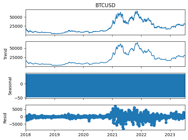

Fourier analysis can be useful in determining frequencies of seasonality. More on this later.

In brief, we can plot the periodogram to determine the strength of different frequencies.

# From https://www.kaggle.com/code/ryanholbrook/seasonality
def plot_periodogram(ts, detrend='linear', ax=None):
    from scipy.signal import periodogram
    fs = pd.Timedelta("365D") / pd.Timedelta("1D")
    freqencies, spectrum = periodogram(
        ts,
        fs=fs,
        detrend=detrend,
        window="boxcar",
        scaling='spectrum',
    )
    if ax is None:
        _, ax = plt.subplots()
    ax.step(freqencies, spectrum, color="purple")
    ax.set_xscale("log")
    ax.set_xticks([1, 2, 4, 6, 12, 26, 52, 104])
    ax.set_xticklabels(
        [
            "Annual (1)",
            "Semiannual (2)",
            "Quarterly (4)",
            "Bimonthly (6)",
            "Monthly (12)",
            "Biweekly (26)",
            "Weekly (52)",
            "Semiweekly (104)",
        ],
        rotation=30,
    )
    ax.ticklabel_format(axis="y", style="sci", scilimits=(0, 0))
    ax.set_ylabel("Variance")
    ax.set_title("Periodogram")
    return ax


plot_periodogram(df['BTCUSD'])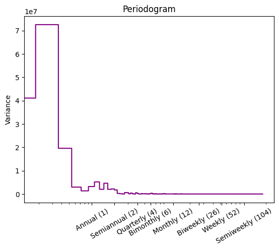

1.4. Stationarity

A stationary time series is one whose properties do not depend on the time at which the series is observed

From Forecasting: Principles and Practice

In other words, the mean and variance do not change over time.

In the context of financial time series, it is often the case that price is non-stationary, but returns (the lag-1 difference) is stationary.

The Augmented Dickey-Fuller test provides a test statistic to quantify stationarity.

Using the BTCUSD time series as an example, the price series is definitely not stationary. We can see this from a plot, but the ADF test corroborates this with a p-value of 0.58.

from statsmodels.tsa.stattools import adfuller

adf_test = adfuller(df['BTCUSD'])
adf_results = {
    "ADF Statistic": adf_test[0],
    "p-value": adf_test[1],
    "Critical Values": adf_test[4],
}

adf_results

{'ADF Statistic': -1.4058608330365159,
 'p-value': 0.5794631585252685,
 'Critical Values': {'1%': -3.4336386745240652,
  '5%': -2.8629927557359443,
  '10%': -2.5675433856598793}}

Next we take the differences. This is stationary, with a tiny p-value.

btc_rets = df['BTCUSD'].diff().dropna()

adf_test = adfuller(btc_rets)
adf_results = {
    "ADF Statistic": adf_test[0],
    "p-value": adf_test[1],
    "Critical Values": adf_test[4],
}

adf_results

{'ADF Statistic': -7.742323245600769,
 'p-value': 1.0538877703747789e-11,
 'Critical Values': {'1%': -3.433643643742798,
  '5%': -2.862994949652858,
  '10%': -2.5675445538118042}}

Time Series Analysis

1. Time Series Properties

1.1. Considerations for Time Series Data

1.2. Trend

1.3. Seasonality

1.4. Stationarity

References