flowchart TD A(Organisation) --> B1(Account 1) A(Organisation) --> B2(Account 2) B1 --> C1(Users) B1 --> C2(Roles) B1 --> C3(Databases) B1 --> C4(Warehouses) B1 --> C5(Other account objects) C3 --> D1(Schemas) D1 --> E1(UDFs) D1 --> E2(Views) D1 --> E3(Tables) D1 --> E4(Stages) D1 --> E5(Other database objects)
1. Overview
The Snowsight interface is the GUI through which we interact with Snowflake.
When querying a Snowflake table, a fully qualified table name means database_name + schema_name + table_name. For example, “DERIVED_DB.PUBLIC.TRADES_DATA”
Worksheets are associated with a role.
A warehouse is needed for compute to execute a query.
Snowflake is a “self-managed cloud data platform”. It is cloud only. No on-premise option.
“Self-managed” service means:
- No hardware
- No software
- No maintenance
“Data platform” means it can function as:
- Data warehouse
- Data lake - mix of structured and semi structured data
- Data science - use your preferred language via Snowpark
2. Snowflake Architecture
2.2. Layers of Snowflake
There are three distinct layers of Snowflake:
- Database storage
- Compressed columnar storage.
- This is stored as blobs in AWS, Azure, GCP etc.
- Snowflake abstracts this away so we just interact with it like a table.
- This is optimised for OLAP (analytical purposes) which is read-heavy, rather than OLTP which is write-heavy.
- Compute
- “The muscle of the system”.
- Query processing.
- Queries are processed using “virtual warehouses”. These are massive parallel processing compute clusters, e.g. EC2 on AWS.
- Cloud services
- “The brain of the system”.
- Collection of services to manage and coordinate components, e.g. the S3 and EC2 instances used in the other two layers.
- The cloud services layer also runs on a compute instance of the cloud provider and is completely handled by Snowflake.
- This layer handles: authentication, access control, metadata management, infrastructure management, query parsing and optimisation. The query execution happens in the compute layer.
2.3. Loading Data into Snowflake
This is covered more extensively in its own section, but this sub-section serves as a brief introduction.
The usual SQL commands can be used to create databases and tables.
CREATE DATABASE myfirstdb
ALTER DATABASE myfirstdb RENAME firstdb
CREATE TABLE loan_payments (
    col1 string,
    col2 string,
);
We can specify a database to use with the USE DATABASE command to switch the active database. This avoids having to use the fully qualified table name everywhere.
USE DATABASE firstdb

COPY INTO loan_payments
FROM s3/… -- The URL to copy from
file_format = (delimiter = “,”,
               skip rows=1,
               type=csv);
2.4. Snowflake Editions
The different Snowflake editions vary by features and pricing. The feature matrix is available on the Snowflake docs.
- Standard
- Complete DWH, automatic data encryption, support for standard and special data types, time travel 1 day, disaster recovery for 7 days beyond time travel, network policies, federated auth and SSO, 24/7 support
- Enterprise
- Multi cluster warehouse, time travel 90 days, materialised views, search optimisation, column-level security, 24 hour early access to new releases
- Business critical
- Additional security features such as customer managed encryption, support for data specific regulation, database failover and fallback
- Virtual private
- Dedicated virtual servers and warehouse, dedicated metadata store. Isolated from all other snowflake accounts.
2.5. Compute Costs
2.5.1. Overview of Cost Categories
Compute costs and storage costs are decoupled and can be scaled separately. “Pay for what you need”.
- Active warehouses
- Used for standard query processing.
- Billed per second (minimum 1 minute).
- Depends on size of warehouse, time and number of warehouses.
- Cloud services
- Behind-the-scenes cloud service tasks.
- Only charged if >10% of warehouse consumption, which is not the case for most customers.
- Serverless
- Used for search optimisation and Snowpipe.
- This is compute that is managed by snowflake, e.g. event-based processing.
These are charged in Snowflake credits.
2.5.2. Calculating Number of Credits Consumed-
The warehouses consume the following number of credits per hour:
| Warehouse Size | Number of Credits |
|---|---|
| XS | 1 |
| S | 2 |
| M | 4 |
| L | 8 |
| XL | 16 |
| 4XL | 128 |
Credits cost different amounts per edition. It also depends on the cloud provider (AWS) and region (US-East-1). Indicative costs for AWS US-East-1 are:
| Edition | $ / Credit |
|---|---|
| Standard | 2 |
| Enterprise | 3 |
| Business Critical | 4 |
2.6 Storage and Data Costs
2.6.1. Storage Types and Costs
Monthly storage costs are based on average storage used per month. Also depends on cloud provider and region. Cost is calculated AFTER Snowflake’s data compression.
There are two options for storage pricing:
- On demand storage: Pay for what you use.
- Capacity storage: Pay upfront for defined capacity.
Typically start with on demand until we understand our actual usage, then shift to capacity storage once this is stable.
2.6.2. Transfer Costs
This depends on data ingress vs egress.
- Data IN is free
- Snowflake wants to remove friction to getting your data in.
- Data OUT is charged
- Snowflake wants to add friction to leaving.
- Depends on cloud provider and region. In-region transfers are free. Cross-region or cross-providers are charged.
2.7. Storage Monitoring
We can monitor storage for individual tables.
SHOW TABLES gives general table storage stats and properties.
We get more detailed views with TABLE_STORAGE_METRICS. We can run this against the information schema or the account storage. These split the sizes into active bytes, time travel bytes and failsafe bytes.
For the information schema metrics:
SELECT * FROM DB_NAME.INFORMATION_SCHEMA.TABLE_STORAGE_METRICS;For the account admin metrics, this needs to use the correct account admin role USE ROLE ACCOUNTADMIN.
SELECT * FROM SNOWFLAKE.ACCOUNT_USAGE.TABLE_STORAGE_METRICS;We can also look at the Admin -> Usage screen in the Snowflake GUI.
2.8. Resource Monitors
Resource monitors help us control and monitor credit usage of individual warehouses and the entire account.
We can set a credit quota which limit the credits used per period. For example, the maximim number of credits that can be spent per month.
We can set actions based on when a percentage of the credit limit is reached. These percentages can be >100%. There are three options for the choice of action:
- Notify
- Suspend and notify (but continue running tasks that have already started)
- Suspend immediately (aborting any running queries) and notify.
We set this using the Usage tab in the ACCOUNTADMIN role in the snowsight UI under Admin -> Usage. Other roles can be granted MONITOR and MODIFY privileges.
We can select a warehouse then filter on different dimensions, for example, distinguishing storage vs compute vs data transfer costs.
To set up a new resource monitor, we give it:
- Name
- Credit quota: how many credits to limit to
- Monitor type: specific warehouse, group of warehouses, or overall account
- Schedule
- Actions
2.9. Warehouses and Multi Clustering
2.9.1. Warehouse Properties
There are different types and sizes of warehouse and they can be multi-clustered.
Types: standard and snowpark-optimised (for memeory-intensive tasks like ML)
Size: XS to XXL. Snowpark type is only M or bigger and consumes 50% more credits
Multi-clustering is good for more queries, i.e. more concurrent users. We scale horizontally so there are multiple small warehouses rather than one big one. They can be in maximised mode (set size) or autoscaled mode (number of nodes scales between predefined min and max)
The autoscaler decides to add warehouses based on the queue, according to the scaling policy.
- Standard
- Favours starting extra clusters.
- Starts a new cluster as soon as there is a query queued.
- Cluster shuts down after 2 to 3 successful checks. A “check” is when the load on the least used node could be redistributed to other nodes.
- Economy
- Favours conserving credits.
- Starts a new cluster once the workload for the cluster would keep it running for > 6 mins.
- Cluster shuts down after 5-6 successful checks.
2.9.2. Creating a Warehouse
To create a warehouse, we need to use the ACCOUNTADMIN, SECURTIYADMIN or SYSADMIN role.
Warehouses can either be created through UI or SQL.
CREATE WAREHOUSE my_wh
WITH
WAREHOUSE_SIZE = XSMALL
MIN_CLUSTER_COUNT = 1
MAX_CLUSTER_COUNT = 3
AUTO_RESUME = TRUE
AUTO_SUSPEND = 300
COMMENT = 'This is the first warehouse'
We can also ALTER or DROP a warehouse in SQL, just like we normally would with DROP TABLE.
DROP WAREHOUSE my_wh;2.10. Snowflake Objects
There is a hierarchy of objects in Snowflake.
An organisation (managed by ORGADMIN) can have multiple accounts (each managed by am ACCOUNTADMIN). These accounts might be by cloud region or department.
Within each account we have multiple account objects: users, roles, databases, warehouses, other objects.
Databases can have multiple schemas.
Schemas can have multiples UDFs, views, tables, stages, other objects.
2.11. SnowSQL
SnowSQL is used to connect to Snowflake via the command line. It needs to be installed on your local machine.
We can execute queries, load and unload data, etc.
3. Loading and Unloading Data
3.1. Stages
Stages are locations used to store data.
From the stage, say an S3 bucket, we can load data from stage -> database. Likewise, we can unload data from database -> stage (S3 bucket).
Stages can be internal (managed by Snowflake) or external (managed by your cloud provider, eg AWS S3).
3.1.1. Internal Stage
An internal stage is managed by Snowflake.
We upload data into an internal stage using the PUT command. By default, files are compressed with gzip and encrypted.
We load it into the database using the COPY INTO command. We can also unload using the COPY INTO command by varying the destination.
There are three types of stage:
- User stage
- Can only be accessed by one user
- Every user has one by default
- Cannot be altered or dropped
- Accessed with
@~
- Table stage
- Can only be accessed by one table
- Cannot be altered or dropped
- Use this to load to a specific table
- Accessed with
@%
- Named stage
CREATE STAGEto create your own- This is then just like any other database object, so you can modify it or grant privileges
- Most commonly used stage
- Accessed with
@
A typical use case for an internal stage is when we have a file on our local system that we want to load into Snowflake, but we don’t have an external cloud provider set up.
3.1.2. External Stage
An external stage connects to an external cloud provider, such as an S3 bucket.
We create it with the CREATE STAGE command as with an internal stage. This creates a Snowflake object that we can modify and grant privileges to.
CREATE STAGE stage_name
  URL='s3://bucket/path/'
We can add CREDENTIALS argument but this would store them in plain text. A better practice is to pass a STORAGE_INTEGRATION argument that points to credentials.
We can also specify the FILE_FORMAT.
3.1.3. Commands For Stages
Some of the most common commands for stages:
LIST- List all files (and additional properties) in the stage.
COPY INTO- Load data into the stage, or unload data from the stage.
SELECT- Query from stage
DESC- Describe the stage. Shows the default values or arguments.
3.2. COPY INTO
This can bulk load or unload data.
A warehouse is needed. Data transfer costs may apply if moving across regions or cloud providers.
3.2.1. Loading Data
Load data from a stage to a table with:
COPY INTO table_name
FROM stage_name
We can specify a file or list of files with the FILES argument.
Supported file formats are:
- csv (default)
- json
- avro
- orc
- parquet
- xml
We can also use the PATTERN argument to match a file pattern with wildcards, e.g. order*.csv
3.2.2. Unloading Data
Unloading data from the table to a stage uses the same syntax:
COPY INTO stage_name
FROM table_name
As with loading, we can specify a file format with the FILE_FORMAT arg, or pass a reusable FILE_FORMAT object.
COPY INTO stage_name
FROM table_name
FILE_FORMAT = ( FORMAT_NAME = 'file_format_name' |
                TYPE = CSV )
3.3. File Format
If the file format is not specified, it defaults to csv. You can see this and other default values by describing the stage with:
DESC STAGE stage_nameWe can overrule the defaults by specifying FILE_FORMAT argument in the COPY INTO command.
A better practice is to use the file_format arg to pass a file_format object such as
FILE_FORMAT = (TYPE = CSV)We create this object with
CREATE FILE FORMAT file_format_name
TYPE = CSV
FIELD_DELIMITER = ‘,’
SKIP_HEADER = 1
We write this file format to a table like manage_db. Then we can reuse it in multiple places when creating the stage or table, loading or unloading data, etc.
3.4. Insert and Update
Insert is the same as standard SQL:
INSERT INTO table_name
VALUES (1, 0.5, 'string')
To only insert specific columns:
INSERT INTO table_name (col1, col2)
VALUES (1, 0.5)
INSERT OVERWRITE will truncate any existing data and insert only the given values. Use with caution! Any previous data is dropped, the table with only have the rows in this command.
Update also works like standard SQL:
UPDATE table_name
SET col1=10
WHERE col1=1
TRUNCATE removes all of the values in the table.
DROP removes the entire table object and its contents.
3.5. Storage Integration Object
This object stores a generated identity for external cloud storage.
We create it as a Snowflake object which constrains the allowed location and grant permissions to it in AWS, Azure etc.
3.6. Snowpipe
The discussion so far has focused on bulk loading, i.e. manual loading of a batch of data.
Snowpipe is used for continuous data loading.
A pipe is a Snowflake object. It loads data immediately when a file appears in blob storage. It triggers a predefined COPY command. This is useful when data needs to be available immediately.
Snowpipe uses serverless features rather than warehouses.
When files are uploaded to an S3 bucket, it sends an event notification to a serverless process which executes the copy command into the Snowflake database.
CREATE PIPE pipe_name
AUTO_INGEST = TRUE
INGESTION = notification integration from cloud storage
COMMENT = string
AS COPY INTO table_name
FROM stage_name
Snowpipe can be triggered by cloud messages or REST API. Cloud messages are for external stages only with that cloud provider. REST API can be internal or external stage.
- Cost is based on “per second per core” of the serverless process.
- Time depends on size and number of files.
- Ideal file size is between 100-250 MB.
Snowflake stores metadata about the file loading. Old history is retained for 14 days. The location of the pipe is stored in a schema in the database.
The schedule can be paused or resumed by altering the pipe.
ALTER PIPE pipe_name
SET PIPE_EXECUTION_PAUSED = True
3.7. Copy Options
These are arguments we can pass to COPY INTO for loading and unloading. Some options only apply to loading and do not apply to unloading.
They are properties of the stage object, so if the arguments are not passed Snowflake will fall back to these default values.
3.7.1. ON_ERROR
- Data Type: String
- Description: Only for data loading. How to handle errors in files.
- Possible Values:
CONTINUE- Continue loading file if errors are found.SKIP_FILE- Skip loading this file if errors are found. This is the default for Snowpipe.SKIP_FILE_<num>- Skip if>= numerrors are found (absolute).SKIP_FILE_<pct>%- Skip if>= pcterrors are found (percentage).ABORT_STATEMENT- Abort loading if an error is found. This is the default for bulk load.
3.7.2. SIZE_LIMIT
- Data Type: Int
- Description: Maximum cumulative size, in bytes, to load. Once this amount of data has been loaded, skip any remaining files.
- Possible Values: Int bytes.
3.7.3. PURGE
- Data Type: Bool
- Description: Remove files from the stage after they have been loaded.
- Possible Values:
FALSE(default) |TRUE
3.7.4. MATCH_BY_COLUMN_NAME
- Data Type: String
- Description: Load semi structured data by matching field names.
- Possible Values:
NONE(default) |CASE_SENSITIVE|CASE_INSENSITIVE
3.7.5. ENFORCE_LENGTH
- Data Type: Bool
- Description: If we have a varchar(10) field, how should we handle data that is too long?
- Possible Values:
TRUE(default) - Raise an errorFALSE- Automatically truncate strings
TRUNCATECOLUMNS is an alternative arg that does the opposite.
3.7.6. FORCE
- Data Type: Bool
- Description: If we have loaded this file before, should we load it again?
- Possible Values:
False(default) |TRUE
3.7.7. LOAD_UNCERTAIN_FILES
- Data Type: Bool
- Description: Should we load files if the load status is unknown?
- Possible Values:
False(default) |TRUE
3.7.8. VALIDATION_MODE
- Data Type: String
- Description: Validate the data instead of actually loading it.
- Possible Values:
RETURN_N_ROWS- Validate the first N rows and returns them (like a SELECT statement would). If there is one or more errors in those rows, raise the first.RETURN_ERRORS- Return all errors in the file.
3.8. VALIDATE
The VALIDATE function validates the files loaded in a previous COPY INTO.
Returns a list of errors from that bulk load. This is a table function, which means it returns multiple rows.
SELECT *
FROM TABLE(VALIDATE(table_name, JOB_ID => ‘_last’))
We can pass a query ID instead of _last to use a specific job run rather than the last run.
3.9. Unloading
The syntax for unloading data from a table into a stage is the same as loading, we just swap the source and target.
COPY INTO stage_name FROM table_nameWe can unload specific rows or columns by using a SELECT statement:
COPY INTO stage_name
FROM (SELECT col1, col2 FROM table_name)
We can pass a FILE_FORMAT object and HEADER args.
We can also specify the prefix or suffix for each file. By default the prefix is data_ and the suffix is _0, _1, etc.
COPY INTO stage_name/myprefixThis is the default behaviour to split the output into multiple files once MAX_FILE_SIZE is reached, setting an upper limit on the output. The SINGLE parameter can be passed to override this, to force the unloading task to keep the output to a single file without splitting.
If unloading to an internal stage, to get the data on your local machine use SnowSQL to run a GET command on the internal stage after unloading.
You can then use the REMOVE command to delete from the internal stage.
4. Data Transformation
4.1. Transformations and Functions
We can specify transformations in the SELECT statement of the COPY command.
This can simplify ETL pipelines when performing simple transformations such as: column reordering, casting data types, removing columns, truncating strings to a certain length. We can also use a subset of SQL functions inside the COPY command. Supports most standard SQL functions defined in SQL:1999.
Snowflake does not support more complex SQL inside the COPY command, such as FLATTEN, aggregations, GROUP BY, filtering with WHERE, JOINs.
Supported functions:
- Scalar functions. Return one value per row. E.g.
DAYNAME - Aggregate functions. Return one value per group / table. E.g.
MAX. - Window functions. Aggregate functions that return one value per row. E.g.
SELECT ORDER_ID, SUBCATEGORY, MAX(amount) OVER (PARTITION BY SUBCATEGORY) FROM ORDERS; - Table functions. Return multiple rows per input row. E.g.
SELECT * FROM TABLE(VALIDATE(table_name, JOB_ID => ‘_last’)) - System functions. Control and information functions. E.g.
SYSTEM$CANCEL_ALL_QUERIES - UDFs. User-defined functions.
- External functions. Stored and executed outside of Snowflake.
4.2. Estimation Functions
Exact calculations on large tables can be very compute-intensive or memory-intensive. Sometimes an estimate is good enough.
Snowflake has some algorithms implemented out of the box that can give useful estimates with fewer resources.
4.2.1. Number of Distinct Values - HLL()
HyperLogLog algorithm.
Average error is ~1.6%.
Replace
COUNT(DISTINCT (col1, col2, ...))with
HLL(col1, col2, ...)or
APPROX_COUNT_DISTINCT (col1, col2, ...)4.2.2. Frequent Values - APPROX_TOP_K()
Estimate the most frequent values and their frequencies. Space-saving algorithm.
Use the following command. The k argument is optional and defaults to 1. The counters argument is optional and specifies the maximum number of distinct values to track. If using this, we should use counters >> k.
APPROX_TOP_K (col1, k[optional], counters[optional])4.2.3. Percentile Values - APPROX_PERCENTILE()
t-Digest algorithm.
APPROX_PERCENTILE (col1, percentile)4.2.4. Similarity of Two or More Data Sets - MINHASH & APPROXIMATE_SIMILARITY()
The full calculation uses the Jaccard similarity cofficient. This returns a value between 0 and 1 indicating similarity. \[ J(A, B) = |(A \cap B)| / |A \cup B| \]
The approximation is a two-step process that uses the MinHash algorithm to hash each table, then the APPROXIMATE_SIMILARITY function to estimate \(J(A, B)\).
The argument k in MINHASH is the number of hash functions to use. Higher k is more accurate but slower. We can pass individual column names instead oif *.
SELECT MINHASH(k, *) AS mh FROM table_name;The full approximation command is:
SELECT APPROXIMATE_SIMILARITY(mh)
FROM (
    SELECT MINHASH(100, *) AS mh FROM mhtab1
    UNION ALL
    SELECT MINHASH(100, *) AS mh FROM mhtab2
);
4.3. User-Defined Functions (UDF)
These are one of several ways of extending functionality with additional functions.
(The other approaches are stored procedures and external functions, which are covered in the next sections.)
UDFs support the following languages: SQL, Python, Java, JavaScript
4.3.1. Defining a UDF
We can define a SQL UDF using create function.
CREATE FUNCTION add_two(n int)
returns int
    AS
    $$
    n+2
    $$;
Defining a UDF in Python is similar, we just need to specify the language and some other options.
CREATE FUNCTION add_two(n int)
returns int
language Python
runtime_version =‘3.8’
handler = ‘addtwo’
    AS
    $$
    def add_two(n):
        return n+2
    $$;
4.3.2. Using a UDF
We just call the UDF from SnowSQL, for example
SELECT add_two(3);4.3.3. Function Properties
Functions can be:
- Scalar functions: Return one output row per input row.
- Tabular functions: Return a table per input row.
Functions are schema-level objects in Snowflake. We can see them under Schema.Public.Functions.
We can manage access and grant privileges to functions, just like any other Snowflake object.
4.4. Stored Procedures
Another way of extending functionality, like UDFs.
UDF vs stored procedures: - UDF is typically used to calculate a value. It needs to return a value. No need to have access to the objects referenced in the function. - A stored procedure is typically used for database operations like INSERT, UPDATE, etc. It doesn’t need to return a value.
Can rely on the caller’s or the owner’s access rights.
Procedures are securable objects like functions, so we can grant access to them.
Supported languages:
- Snowflake scripting - Snowflake SQL + procedural logic
- JavaScript
- Snowpark API - Python, Scala, Java
4.4.1. Creating a Stored Procedure
CREATE PROCEDURE find_min(n1 int, n2 int)
returns int
language sql
    AS
    BEGIN
    IF (n1 < n2)
        THEN RETURN n1;
        ELSE RETURN n2;
    END IF;
    END;
Stored procedures can be run with the caller’s rights or the user’s rights. This is defined with the stored procedure. By default, they run as owner but we can override this with:
execute as caller4.4.2. Calling a Stored Procedure
CALL find_min(5,7)We can reference dynamic values, such as variables in the user’s sessions, in stored procedures. - If argument is referenced in SQL, use :argname - If an object such as a table is referenced, use IDENTIFIER(:table_name)
4.5. External Functions
These are user-defined functions that are stored and executed outside of Snowflake. Remotely executed code is referred to as a “remote service”.
This means it can reference third-party libraries, services and data.
Examples of external API integrations are: AWS lambda function, Microsoft Azure function, HTTPS server.
CREATE EXTERNAL FUNCTION my_func(string_col VAR_CHAR)
returns variant
api_integration = azure_external_api_integration
AS 'https://url/goes/here'
Security-related information is stored in an API integration. This is a schema-level object, so it is securable and can be granted access to .
Advantages:
- Can use other languages
- Access 3rd-party libraries
- Can be called from elsewhere, not just Snowflake, so we can have one central repository.
Limitations:
- Only scalar functions
- Slower performance - overhead of external functions
- Not shareable
4.6. Secure UDFs and Procedures
We may want to hide certain information such as the function definition, or prevent users from seeing underlying data.
We just use the SECURE keyword.
CREATE SECURE FUNCTION ...Disadvantages: - Lower query performance. The optimiser exposes some security risks, so this is locked down which restricts the optimisation options available therefore impacting performance lock this down the optimisations are restricted.
We should use it for sensitive data, otherwise the performance trade-off isn’t worthwhile.
4.7. Sequences
Sequences are typically used for DEFAULT values in CREATE TABLE statements. Sequences are not guaranteed to be gap-free.
Sequences are securable objects that we can grant privileges to.
It is a schema object like: Functions, Stored Procedures, Tables, File Formats, Stages, Stored Procedures, UDFs, Views, and Materialized Views.
CREATE SEQUENCE my_seq
START = 1
INCREMENT = 1
Both START and INCREMENT default to 1.
We invoke a sequence with my_seq.nextval. For example:
CREATE TABLE my_table(
    id int DEFAULT my_seq.nextval,
    first_name varchar
    last_name varchar
);

INSERT INTO my_table(first_name, last_name)
VALUES ('John', 'Cena'), ('Dwayne', 'Johnson'),('Steve','Austin');
4.8. Semi-structured Data
4.8.1. What is Semi-structured Data?
Semi-structured data has no fixed schema, but contains tags/labels and has a nested structure.
This is in contrast to structured data like a table. Or unstructured data which is a free-for-all.
Supported formats: json, xml, parquet, orc, avro
Snowflake deals with unstructured data using 3 different data types:
- Object - think of this in the JavaScript sense, i.e. key:value pairs
- Array
- Variant - this can store data of any other type, including arrays and objects. Native support for semi-structured data.
We typically let Snowflake convert semi-structured data into a hierarchy of arrays and objects within a variant object.
Nulls and non-native strings like dates are cast to strings within a variant.
Variant can store up to 16 MB uncompressed per row. If the data exceeds this, we will need to restructure or split the input.
The standard “ELT” approach (Extract, Load, Transform) for semi-structured data is to load the data as is, then transform it later once we’ve eyeballed it. This is a tweak of the classic ETL approach.
We often need to FLATTEN the data.
4.8.2. Querying Semi-structured Data
To access elements of a VARIANT column, we use a :.
For example, if the raw_column column has a top-level key of heading1, we can query:
SELECT raw_column:heading1
FROM table_with_variant
We can also refer to columns by their position. So to access the first column:
SELECT $1:heading1
FROM table_with_variant
To access nested elements, use .:
SELECT raw_column:heading1.subheading2
FROM table_with_variant
If there is an array, we can access elements of the array with [index]. Arrays are 0-indexed, so to access the first element:
SELECT raw_column:heading1.subheading2.array_field[0]
FROM table_with_variant
We may also need to cast the types of the element with ::
SELECT raw_column:heading1.subheading2.array_field[0]::VARCHAR
FROM table_with_variant
4.8.3. Flatten Hierarchical Data
We may want to flatten the hierarchies within semi-structured datainto a relational table. We do this with the FLATTEN table function.
FLATTEN(INPUT => <expression>)Note that FLATTEN cannot be used inside a COPY command.
We can use it alongside the other keys of the data. For example:
SELECT
    RAW_FILE:id,
    RAW_FILE:first_name,
    VALUE as prev_company  -- this is the flatten array
FROM
    MY_DB.PUBLIC.JSON_RAW_TABLE,
    TABLE(FLATTEN(input => RAW_FILE:previous_companies))
There is an implicit lateral join between the table and the flattened table function result set. We can make this explicit using the LATERAL FLATTEN keywords. The result is the same.
4.8.4. Insert JSON Data
We use the PARSE_JSON function to import JSON data.
SELECT PARSE_JSON(' { "key1": "value1", "key2": "value2" } ');When inserting variant data, we don’t use INSERT VALUES, we use a SELECT statement.
INSERT INTO semi_structured_table_name
SELECT PARSE_JSON(' { "key1": "value1", "key2": "value2" } ');
4.9. Unstructured Data
Unstructured data is any data which does not fit in a pre-defined data model. E.g. video files, audio files, documents.
Snowflake handles unstructured data using file URLs.
Snowflake supports the following for both internal and external stages:
- Access through URL in cloud storage
- Share file access URLs
4.9.1. File URLs
There are three types of URL we can share:
| URL Type | Use Case | Expiry | Command to Return URL |
|---|---|---|---|
| Scoped URL | Encoded URL with temporary access to a file but not the stage. | Expires when results cache expires (currently 24 hours) | BUILD_SCOPED_FILE_URL |
| File URL | Permits prolonged access to a specified file. | Does not expire. | BUILD_STAGE_FILE_URL |
| Pre-signed URL | HTTPS URL used to access a file via a web browser. | Configurable expiration time for access token. | GET_PRESIGNED_URL |
For example, run the following SQL file function to create a scope URL:
SELECT BUILD_SCOPED_FILE_URL(@stage_azure, 'Logo.png')For a pre-signed URL, we also set the expiry time in seconds.
SELECT GET_PRESIGNED_URL(@stage_azure, 'Logo.png', 60)4.9.2. Directory Tables
A directory table stores metadata of staged files.
This is layered on a stage, rather than being a separate table object in a database.
It can be queried, with sufficient privileges on the stage, to retrieve file URLs to access files on the stage.
It needs to be enabled as it is not by default. We either do this in the CREATE STAGE command with
CREATE STAGE stage_azure
URL = <'url'>
STORAGE_INTEGRATION = integration
DIRECTORY = (ENABLE = TRUE)
or ALTER an existing stage:
ALTER STAGE stage_azure
SET DIRECTORY = (ENABLE = TRUE)
We query this directory with:
SELECT * FROM DIRECTORY(@stage_azure)The first time querying, so will not see any results. The directory needs to be manually populated with:
ALTER STAGE stage_azure REFRESHWe may want to use the cloud provider’s event notification to set up an automatic refresh.
4.10. Data Sampling
When developing views and queries against large databases, it may take a lot of time/compute to query against the entire database, making it slow to iterate. So we often want to work with a smaller subset of the data.
Use cases:
- Query development
- Data analysis, estimates
There are two sampling methods:
- The
ROW/BERNOULLImethod (both keywords give identical results). The following command will sample 10% of rows. We can optionally add aSEED(69)argument to get reproducible results.
SELECT * FROM table
SAMPLE ROW(10)
SEED(69)- The
BLOCK/SYSTEMmethod
SELECT * FROM table
SAMPLE BLOCK(10)
SEED(69)
Comparison of row vs block sampling:
ROW |
BLOCK |
|---|---|
| Every row has probability \(p\) of being chosen | Every block (i.e. micro partition in block storage) has probability \(p\) of being chosen |
| More randomness | More efficient processing |
| Better for smaller tables | Better for larger tables |
4.11. Tasks
Tasks are used to schedule the execution of SQL statements or stored procedures. The are schema-level objects, so can be cloned.
They are often combined with streams to set up continuous ETL workflows.
CREATE TASK my_task
    WAREHOUSE = my_wh
    SCHEDULE = '15 MINUTE'
    AS
    INSERT INTO my_table(time_col) VALUES (CURRENT_TIMESTAMP);
If we omit the WAREHOUSE argument, the task will run using Snowflake-managed compute.
The task is run using the privileges of the task owner.
To create a new task we need the following privileges: EXECUTE MANAGED TASK on account, CREATE TASK on schema and USAGE on warehouse.
To start/stop a task, we use the following commands. We always need to RESUME a task the first time we use it after creating it.
ALTER TASK my_task RESUME;
ALTER TASK my_task SUSPEND;
As well as setting up individual tasks, we can set up a DAG of interconnected tasks. We specify the dependencies using the AFTER keyword. DAGs are limited to 1000 tasks in total and 100 child tasks for a single node.
CREATE TASK my_task_b
    WAREHOUSE = my_wh
    AFTER mytask_a
    AS
    ...
4.12. Streams
A stream is an object which records Data Manipulation Language (DML) changes made to a table. This is change data capture. It is a schema-level object and can be cloned. The stream will be cloned when a database is cloned.
If a stream is set up on a table, the stream will record any inserts, deletes, updates to the table. We can then query the stream to see what has changed.
To create a stream:
CREATE STREAM my_stream
ON TABLE my_table;
We can query from the stream. This will return any changed rows along with three metadata columns: METADATA$ACTION, METADATA$ISUPDATE, METADATA$ROW_ID.
SELECT * FROM my_stream;Consuming a stream means we query its contents and then empty it. This is a typical use case in ETL work flows where we want to monitor for deltas and update another table. We do this by inserting into a target table from the stream:
INSERT INTO target_table
    SELECT col1, col2
    FROM my_stream;
Three types of stream:
- Standard: Insert, update, delete.
- Append-only: Insert. Does not apply to external tables, only standard tables, directory tables, views.
- Insert-only: Insert. Only applies to external tables.
A stream becomes stale when the offset is outside the data retention period of the table, i.e. unconsumed records in the stream are lost.
This determines how frequently a stream should be consumed. The STALE_AFTER column of DESCRIBE STREAM or SHOW STREAMS indicated when the stream is predicted to go stale.
A stream extends the data retention period of the source table to 14 days by default. This is true for all snowflake editions. This is the MAX_DATA_EXTENION_TIME_IN_DAYS variable which defaults to 14 and can be increased to 90.
To trigger a task when a stream has data using WHEN SYSTEM$STREAM_HAS_DATA. For example:
CREATE TASK my_task
    WAREHOUSE = my_wh
    SCHEDULE = '15 MINUTE'
    WHEN SYSTEM$STREAM_HAS_DATA('my_stream')
    AS
    INSERT INTO my_table(time_col) VALUES (CURRENT_TIMESTAMP);
5. Snowflake Tools and Connectors
5.1. Connectors and Drivers
Snowflake provides two interfaces:
- Snowsight web UI
- SnowSQL command line tool
Drivers:
- Go
- JDBC
- .NET
- node.js
- ODBC
- PHP
- Python
Connectors:
- Python
- Kafka
- Spark
Partner Connect allows us to create a trial account for third-party add-ons to Snowflake and integrate them with Snowflake.
They span many different categories and tools - BI, CI/CD, etc.
5.2. Snowflake Scripting
Mostly used in stored procedures but can also be used for writing procedural code outside of this.
We can use@ if, case, for, repeat, while, loop
This is written in a “block”:
DECLARE
BEGIN
EXCEPTION
END
DECLARE and EXCEPTION are optional.
This is available in Snowsight. The classic UI or SnowSQL requires $$ around the block.
Objects created in the block are available outside of it too. Variables created in the block can only be used inside it.
This is a similar syntax, but different from transactions which use BEGIN and END.
5.3. Snowpark
Snowpark API provides support for three programming languages: Python, Java, Scala.
Python code converts to SQL which then queries Snowflake with serverless Snowflake engine.
This means there is no need to move data outside of Snowflake.
Benefits:
- Lazy evaluation
- Pushdown - query is executed in Snowflake rather than unloading all data outside of Snowflake and then transforming
- UDFs can be defined inline
6. Continuous Data Protection
This section covers the data protection lifecycle. From most accessible to least accessible:
flowchart LR

  A(Current data storage) --> B(Time travel) --> C(Fail safe)
6.1. Time Travel
What if someone drops a database or table accidentally? We need a backup to recover data. Time travel enables accessing historical data.
We can:
- Query data that has been deleted or updated
- Restore dropped tables, schemas and databases
- Create clones of tables, schemas and databases from a previous date
We can use a SQL query to access time travel data within a retention period. The AT keyword allows us to time travel.
SELECT *
FROM table
AT (TIMESTAMP >= timestamp)
Or use OFFSET in seconds. So for 10 minutes:
SELECT *
FROM table
AT (OFFSET >= 10*60)
Alternatively we can use BEFORE, where query_ID is the ID where we messed things up:
SELECT *
FROM table
BEFORE (STATEMENT>= query_id)
Go to Activity -> Query History in the Snowsight UI to get the correct query ID.
It is best practice to recover to an intermediate backup table first to confirm the recovered version is correct. E.g.
CREATE OR REPLACE TABLE table_name_backup
FROM table
AT (TIMESTAMP >= timestamp)
6.2. UNDROP
We can use the UNDROP keyword to recover objects.
UNDROP TABLE table_nameSame for SCHEMA or DATABASE.
Considerations.
- UNDROP fails if an object with the same name already exists.
- We need ownership privileges to UNDROP an object.
When working with time zones, it can be helpful to change the time zone to match your local time. This only affects the current session, not the whole account.
ALTER SESSION SET TIMEZONE = 'UTC'6.3. Retention Period
Retention period is the number of days for which historical data is preserved. This determines how far back we can time travel.
The retention period is configurable for table, schema, database or account.
The default DATA_RETENTION_TIME_IN_DAYS=1. If we want to disable time travel, we can set this to 0.
We can set this when we create a table, or alter it for an existing table:
ALTER TABLE table_name (
    SET DATA_RETENTION_TIME_IN_DAYS=2
)
We can set a minimum value at the account level:
ALTER ACCOUNT SET
MIN_DATA_RETENTION_TIME_IN_DAYS=3
The account type determines the maximum retention period:
- Standard: up to 1 day
- Enterprise or higher: up to 90 days
6.4. Fail Safe
This is for disaster recovery beyond time travel. This is not configurable and set to 7 days beyond time travel period for permanent tables.
We as users cannot access this data. We have to contact Snowflake support to restore it for us.
6.5. Storage Costs
Time travel and fail safe contribute to storage costs. You only pay for what is modified.
You can see the breakdown in the Admin -> Usage tab of the UI.
You can see how much storage is being used with:
SELECT *
FROM SNOWFLAKE_ACCOUNT_USAGE.TABLE_STORAGE_METRICS
6.6. Table Types
The following table summarises the differences between the 3 types of table.
| Table Type | Command | Time Travel Retention Period | Fail Safe | Use Case |
|---|---|---|---|---|
| Permanent | CREATE TABLE | 0-90 | Y | Standard tables. Persist data until dropped. |
| Transient | CREATE TRANSIENT TABLE | 0-1 | N | For large tables that do not need to be protected. Persist data until dropped. |
| Temporary | CREATE TEMPORARY TABLE | 0-1 | N | Non-permanent data just for this session.Only in session - data is deleted after the worksheet is closed. |
These types are also available for other Snowflake objects: tables, stages, schema, database.
If a database is transient, so are all of its objects.
Temporary table names do not clash with permanent or transient tables. The temporary table name takes precedence in the session and hides the others with the same name.
It is not possible to change the type of an existing object.
7. Zero-Copy Cloning and Sharing
7.1. Zero Copy Cloning
Zero copy cloning makes it easy to copy an existing object in a storage-efficient way.
For example:
CREATE TABLE table_name
CLONE table_source
We can clone almost* any object: database, schema, table, stream, file format, sequence, task, stage, pipe.
*the exceptions are:
- pipes which can only be cloned if referencing an external stage
- stages which cannot be cloned for named internal stages
When we clone a database or schema, all of its child objects are also cloned.
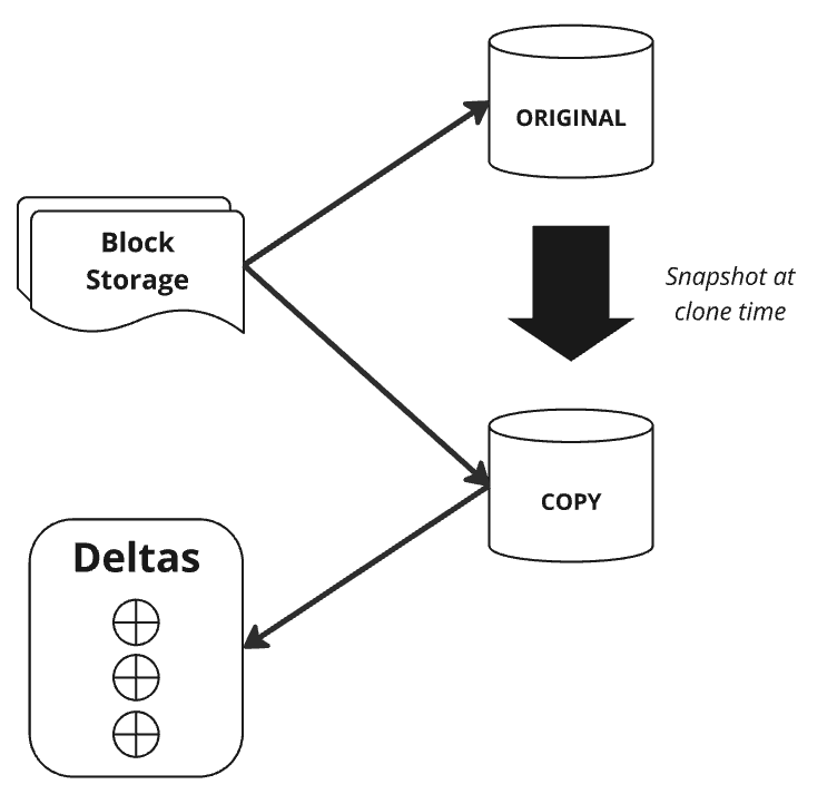
It’s called a “zero copy clone” because it does not actually copy the data at clone time. It is a metadata operation occurring in the cloud service layer.
The “copy” is a snapshot of the “original”. Both reference the same underlying micro-partitions in block storage. Think of it like pass-by-reference rather than pass-by-value.
When modifying the “copy” Snowflake only stores the deltas, not the entire database again. The “original” and “copy” can be modified independently without affecting the other.
A typical use case is to create backups for dev work.
We can clone from a time travel version of a table:
CREATE TABLE table_new
CLONE table_source
BEFORE (TIMESTAMP >= ‘2025-01-31 08:00:00’)
7.2. Privileges
The privileges of the CHILD objects are inherited from the clone source if it is a container like a table or schema. But the privileges of the cloned object itself are NOT inherited. They need to be specified separately by the administrator.
The privileges required to clone an object depends on the object:
- Table: SELECT privileges
- Pipe, stream, task: OWNER privileges
- All other objects: USAGE privileges
When we clone a table, its load history metadata is NOT copied. This means loaded data can be loaded again without causing a metadata clash.
7.3. Data Sharing
7.3.1. What is a Data Share?
Data sharing can usually be quite complicated; managing multiple extracts of a common database and ensuring they are in sync.
Snowflake separates storage vs compute. This allows us to share data without actually making a copy of it. As with zero copy cloning, this is a metadata operation, so uses the cloud service layer.
We grant access to the storage, and the customer provides their own compute resources.
This is available for all Snowflake pricing tiers.
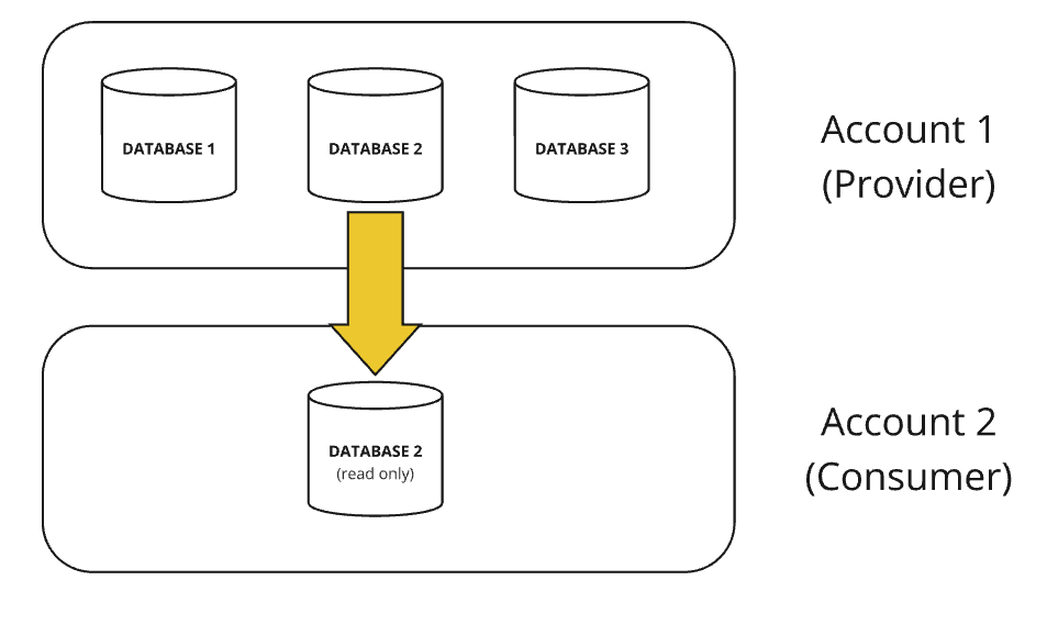
In a one-way data share, Account 1 is the provider and Account 2 is the Consumer. Account 2 has a read-only view of the shared data. The provider is billed for the storage, whereas the consumer is billed for the compute costs of their queries.
An account can be simultaneously both a provider and consumer of data. You can even do this within the same account.
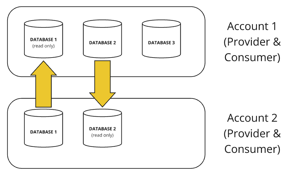
A share contains a single database. We can add multiple accounts to a share.
7.4. Database Replication
Data shares are only possible within the same region and the same cloud provider.
Database replication allows us to share data across different regions or on different cloud providers. It replicates a database between accounts within the same organisation. Also called “cross-region sharing”. This is available at all price tiers.
This incurs data transfer costs because it does actually copy the data across to a different location. The data and objects therefore need to be synchronised periodically.
The provider is referred to as the primary database and the consumer is the secondary database or a read-only replica.
To set up database replication we need to:
- Enable this at the account level with the ORGADMIN role.
SELECT system$global_account_set_parameter(org_name.account_name), 'ENABLE_ACCOUNT_DATABASSE_REPLICATION', 'true');- Promote a local database to primary database with ACCOUNTADMIN role.
ALTER DATABASE my_db ENABLE REPLICATION TO ACCOUNTS myorg.account2, myorg.account3;- Create a replica in the consumer account.
CREATE DATABASE my_db AS REPLICA OF myorg.account1.my_db- Refresh the database periodically. Ownership privileges are needed. We may want to set up a task to run this periodically.
ALTER DATABASE my_db REFRESH;8. Account and Security
8.1. Access Control
There are two approaches to access control:
- Discretionary Access Control (DAC)
- Each object has an owner. That owner can grant access to the object.
- Role-based Access Control (RBAC)
- Privileges are assigned to objects. Those privileges can be granted to roles. These roles can be assigned to users.
We do not assign privileges directly to users.
flowchart LR

A(Object) --> B(Privilege) --> C(Role) --> D(User)
Key concepts:
- Securable object: An object that access can be granted to. Access is denied unless explicitly granted.
- Privilege: A defined level of access.
- Role: The entity to which privileges are granted. Roles can be assigned to users or other roles. We can create a hierarchy of roles.
- User: The identity associated with a person or program.
We can GRANT privileges to a role:
GRANT my_privilege
ON my_object
TO my_role
And GRANT a role to a user.
GRANT my_role
TO user_id
We can also grant access to all tables in a schema:
GRANT SELECT
ON ALL TABLES IN SCHEMA MARKETING_SALES
TO ROLE MARKETING_ADMIN
And also all future tables too:
GRANT SELECT
ON FUTURE TABLES IN SCHEMA MARKETING_SALES
TO ROLE MARKETING_ADMIN
We can REVOKE privileges in the same way:
REVOKE privilege
ON object
FROM role
8.2. Roles
A role is an entity that we assign privileges to.
Roles are then assigned to users. Multiple roles can be assigned to each user.
We need to grant access to all parent objects. So if we want to grant SELECT access to a table, we also need to grant USAGE access to the parent schema and database.
Every object is owned by one single role. Ownership can be transferred.
The SHOW ROLES command shows all available roles.
There is a “current role” used in every session. USE ROLE can be used in Snowflake worksheets or tasks.
8.2.1. System-Defined Roles
These roles can’t be dropped. Additional privileges can be added to the roles, but not revoked.
The roles inherit from parent roles in the hierarchy.
It is best practice for custom roles to inherit from the SYSADMIN role.
ORGADMIN- Manage actions at the organisation level.
- Create and view accounts.
ACCOUNTADMIN- Top-level in hierarchy.
- Should only be grant to a limited number of users as it is the most powerful. It can manage all objects in the account.
- We can create reader accounts and shares. Modify account level parameters including billing and resource monitors.
- Contains SECURITYADMIN AND SYSADMIN roles.
SECURITYADMIN- Manage any object grants globally.
MANAGE GRANTSprivilege.- Create, monitor and manage users and roles.
- Inherits from USERADMIN. The difference with USERADMIN is SECURITYADMIN can manage grants GLOBALLY.
SYSADMIN- Manages objects - it can create warehouses, databases and other objects.
- All custom roles should be assigned to SYSADMIN so that SYSADMIN always remains a superset of all other roles and can manage any object by them.
USERADMIN- For user and role management.
CREATE USERandCREATE ROLEprivileges.
PUBLIC- Automatically granted by default.
- Granted when no access control is needed. Objects can be owned but are available to everyone.
CUSTOM- Can be created by USERADMIN or higher.
- CREATE ROLE privilege. Should be assigned to SYSADMIN so that they can still manage all objects created by the custom role. Custom roles can be created by the database owner.
8.2.2. Hierarchy of Roles
There is a hierarchy of roles.
flowchart BT

F(PUBLIC) --> E(USERADMIN) --> D(SECURITYADMIN) --> A(ACCOUNTADMIN)
C1(Custom Role 1) --> B(SYSADMIN) --> A(ACCOUNTADMIN)
C3(Custom Role 3) --> C2(Custom Role 2) --> B(SYSADMIN)
This is similar to the hierarchy of objects that we’ve seen before in Section 2.10.
8.3. Privileges
Privileges define granular level of access to an object.
We can GRANT and REVOKE privileges. The owner of an object can manage its privileges. The SECURITYADMIN role has the global MANAGE GRANTS privilege, so can manage privileges on any object.
We can see all privileges in the Snowflake docs.
Some of the important ones below.
Global privileges:
- CREATE SHARE
- IMPORT SHARE
- APPLY MASKING POLICY
Virtual warehouse:
- MODIFY - E.g. resizing
- MONITOR - View executed queries
- OPERATE - Suspend or resume
- USAGE - Use the warehouse to execute queries
- OWNERSHIP - Full control over the warehouse. Only one role can be an owner.
- ALL - All privileges except ownership
Databases:
- MODIFY -
ALTERproperties of the database - MONITOR - Use the
DESCRIBEcommand - USAGE - Query the database and execute
SHOW DATABASEScommand - REFERENCE_USAGE - Use an object (usually secured view) to reference another object in a different database
- OWNERSHIP - Full control
- ALL - Everything except ownership
- CREATE SCHEMA
Stages:
- READ - Only for internal stages. Use GET, LIST, COPY INTO commands
- WRITE - Only for internal stages. Use PUT, REMOVE, COPY INTO commands
- USAGE - Only for external stages. Equivalent of read and write.
- ALL
- OWNERSHIP
Tables:
- SELECT
- INSERT
- UPDATE
- DELETE
- TRUNCATED
- DELETE
- ALL
- OWNERSHIP
We can see the grants of a role with:
SHOW GRANTS TO ROLE MARKETING_ADMINWe can see which users are assigned to a role with
SHOW GRANTS OF ROLE MARKETING_ADMIN8.4. Authentication
Authentication is proving that you are who you say you are.
Snowflake uses Multi-Factor Authentication (MFA). This is powered by Duo, managed by Snowflake. MFA is available for all Snowflake editions and is supported by all Snowflake interfaces: web UI, SnowSQL, ODBC and JDBC, Python connectors.
Enabled by default for accounts but requires users to enroll. Strongly recommended to use MFA for ACCOUNTADMIN.
The SECURITYADMIN or ACCOUNTADMIN roles can disable MFA for a user.
We can enable MFA token caching to reduce the number of prompts. This needs to be enabled; it isn’t by default. It makes the MFA token valid for 4 hours. Available for ODBC driver, JDBC driver and Python connector.
8.5. SSO
Federated authentication enables users to login via Single Sign-On (SSO).
The federated environment has two components:
- Service provider: Snowflake
- External identity provider: Maintains credentials and authenticates users. Native support for Okta and Microsoft AD FS. Most SAML 2.0 compliant vendors are supported.
Workflow for Snowflake-initiated login:
- User navigates to web UI
- Choose login via configured Identity Provider (IdP)
- Authenticate via IdP credentials
- IdP sends a SAML response to Snowflake
- Snowflake opens a new session
Workflow for IdP-initiated login:
- User navigates to IdP
- Authenticate via IdP credentials
- Select Snowflake as an application
- IdP sends a SAML response to Snowflake
- Snowflake opens a new session
IdP has SCIM support. This is an open standard for automating user provisioning. We can create a user in the IdP and this provisions the user in Snowflake.
8.6. Key-Pair Authentication
Enhanced security as an alternative to basic username and password.
User has a public key and a private key. This is the key-pair. Minimum key size is 2048-bit RSA key-pair.
Setting this up:
- Generate private key
- Generate public key
- Store keys locally
- Assign public key to user. See command below.
- Configure client to use key-pair authentication
We can set the public key for a user with:
ALTER USER my_user SET
RSA_PUBLIC_KEY 'Fuak_shakfjsb';
8.7. Column-level Security
Column-level security masks data in tables and views enforced on columns.
This is an enterprise edition feature.
8.7.1. Dynamic Data Masking
With “dynamic data masking” the unmasked data is stored in the database, then depending on the role querying the data it is masked at runtime.
We can define a masking policy with:
CREATE MASKING POLICY my_policy
AS (col1 varchar) RETURNS varchar ->
    CASE
    WHEN CURRENT ROLE IN (role_name)
    THEN col1
    ELSE “##-##”
    END;
We apply a masking policy with:
ALTER TABLE my_table MODIFY COLUMN phone;We can remove the policy with:
UNSET MASKING POLICY my_policy;8.8. External Tokenisation
Data is tokenised.
The benefit is the analytical value is preserved; we can still group the data and draw conclusions, it’s just anonymised. Sensitive data is protected.
The tokenisation happens in a pre-load step and the detokenisation happens at query runtime.
8.9. Row-level Security
Row access policies allow us to determine which rows are visible to which users.
This is only available in the enterprise edition.
Rows are filtered at runtime on a given condition based on user or role.
Define the policy with:
CREATE ROW ACCESS POLICY my_policy
AS (col1 varchar) returns Boolean ->
    CASE
    WHEN current_role() = 'EXAMPLE_ROLE'
    AND col1 = 'value1' THEN true
    ELSE false
    END;
Apply the policy with:
ALTER TABLE my_table ADD ROW POLICY my_policy
ON (col1);
8.10. Network Policies
Network policies allow us to restrict access to accounts based on the user’s IP address. We can also specify ranges of addresses.
This is available in all Snowflake editions.
We can either whitelist or blacklist IP addresses. If an address is in both, the blacklist takes precedence and the IP address is blocked.
To create a network policy we need the SECURITYADMIN role since this has the global CREATE NETWORK POLICY privilege.
CREATE NETWORK POLICY my_network_policy
ALLOWED_IP_LIST = ('192.168.1.95', '192.168.1.113'),
BLOCKED_IP_LIST = ('192.168.1.95')  -- Blacklist takes precedence
To apply this to an account, we again need the SECURITYADMIN role. This is a bit of an exception because this is a change to the account but we don’t need to be ACCOUNTADMIN.
ALTER ACCOUNT SET NETWORK_POLICY;We can also alter a USER instead of an ACCOUNT if we have ownership of the user and the network policy.
8.11. Data Encryption
All data is encrypted at rest and in transit.
This is in all editions and happens automatically by default.
8.11.1. Encryption at Rest
Relevant to data in tables and internal stages. AES 256-bit encryption managed by Snowflake.
New keys are generated for new data every 30 days. Data generated with the old key will still use that old key. Old keys are preserved as long as there is still data that uses them; if not they are destroyed.
We can manually enable a feature to re-key all data every year. This is in the enterprise edition.
8.11.2. Data in Transit
This is relevant for all Snowflake interfaces: WebUI, SnowSQL, JDBc, ODBC, Python Connector. TLS 1.2 end-to-end encryption.
8.11.3. Other Encryption Features
We can additionally enable client-side encryption in external stages.
“Tri-secret secure” enables customers to use their own keys. It is a business-critical edition feature. There is a composite master key which combines this customer-managed key with a Snowflake-managed key.
8.12. Account Usage and Information Schema
These are functions we can use to query object metadata and historical data usage.
The ACCOUNT_USAGE schema is available in the SNOWFLAKE database, which is a shared database available to all accounts. The ACCOUNTADMIN can see everything. There are object metadata views like COLUMNS, and historical usage data views like COPY_HISTORY. The data is not real-time; there is a lag of 45 mins to 3 hours depending on the view. Retention period is 365 days. This does include dropped objects so can include a DELETED column.
READER_ACCOUNT_USAGE lets us query object metadata and historical usage data for reader accounts. It is more limited.
The INFORMATION_SCHEMA is a default schema available in all databases. This is read-only data about the parent database and account-level information. The output depends on which privileges you have. There is a lot of data returned so it can return messages saying to filter the query down. Shorter retention period: 7 days to 6 months. This is real-time, there is no delay. Does not include dropped objects.
8.13. Release Process
Releases are weekly with no downtime.
- Full releases: New features, enhancements, fixes, behaviour changes
- Behaviour changes are monthly (i.e. every 4 weekly releases)
- Patch releases: Bugfixes
Snowflake operate a three stage release approach:
- Day 1: early access for enterprise accounts who request this
- Day 1/2: regular access for standard accounts
- Day 2: final access for enterprise or higher accounts
9. Performance Concepts
9.1. Query Profile
This is a graphical representation of the query execution. This helps us understand the components of the query and optimise its performance.
9.1.1. Accessing Query History
There are three ways to view the query history:
In Snowsight. This is in the
Activity -> Query Historytab, or the Query tab in a worksheet for the most recent query.Information schema
SELECT * FROM TABLE(INFORMATION_SCHEMA.QUERY_HISTORY())
ORDER BY START_TIME;- Account usage schema
SELECT * FROM SNOWFLAKE.ACCOUNT_USAGE.QUERY_HISTORY;9.1.2. The Graphical Representation of a Query
The “Operator Tree” is a graphical representation of the “Operator Types”, which are components of query processing. We can also see the data flow, i.e. the number of records processed. The is also a percentage on each node indicating the percentage of overall execution time.
The “Profile Overview” tab gives details of the total time taken. The “Statistics” tab shows number of bytes scanned, percentage from cache, number of paritions scan.
9.1.3. Data Spilling
It also shows “data spilling”, when the data does not fit in memory and is therefore written to the local storage disk. This is called “spilling to disk”. If the local storage is filled, the data is further spilled to remote cloud storage. This is called “spilling to cloud”.
To reduce spilling, we can either run a smaller query or use a bigger warehouse.
9.2. Caching
There are three mechanisms for caching:
- Result cache
- Data cache
- Metadata cache
If the data is not in a cache, it is retrieved from storage, i.e. the remote disk.
9.2.1. Result Cache
Stores the results of a query. This happens in the cloud service layer.
The result is very fast and avoids re-execution.
This can only happen if:
- The table data and micro-partitions have not changed,
- The query does not use UDFs or enternal functions
- Sufficient privileges and results are still available (cache is valid for 24 hours)
Result caching is enabled by default, but can be disabled using the USE_CACHED_RESULT parameter.
The result cache is purged after 24 hours. If the query is re-run, it resets the purge timer, up to a maximum of 31 days.
9.2.2. Data Cache
The local SSD disk of the virtual warehouse. This cannot be shared with other warehouses.
It improves the performance of subsequent queries which use the same underlying data. We can therefore improve performance and costs by using the same warehouse for queries on similar data.
The data cache is purged if the warehouse is suspended or resized.
9.2.3. Metadata cache
Stores statistics for tables and columns in the cloud services layer.
This is also known as the “metadata store”. The virtual private Snowflake edition allows for a dedicated metadata store.
The metadata cache stores results about the data, such as range of values in a micro-partition, count rows, count distinct values, max/min values. We can then query these without using the virtual warehouse.
This is used for functions like DESCRIBE and other system-defined functions.
9.3. Micro Partitions
The data is cloud storage is stored in micro partitions.
These are chunks of data, usually about 50-500MB in uncompressed size (although they are compressed by Snowflake). The most efficient compression algorithm for each micro partition is used independently.
This is specific to Snowflake’s architecture.
Data is stored in a columnar form. We can improve read queries by only selecting required columns.
Micro partitions are immutable - they cannot be changed once created. New data will be stored in new micro partitions, so the partitions depend on the order of insertion.
9.3.1. Partition Pruning
Micro partitions allow for very granular partition pruning. When we run a query on a table, we can eliminate unnecessary partitions.
Snowflake stores metadata per micro partition. E.g. range of values, number of distinct values, and other properties for query optimisation.
Snowflake optimises queries by using the metadata to determine if a micro partition needs to be read, so it can avoid reading all of the data.
9.3.2. Clustering Keys
Clustering keys let us influence how the data is partitioned. This helps improve query performance by improving partition pruning. Grouping similar rows in micro-partitions also generally improves column compression.
Clustering a table on a specific column redistributes the data in the micro-partitions.
Snowflake stored metadata about the micro-partitions in a table:
- Number of micro-partitions
- Overlapping micro-partitions: Number of partitions with overlapping values
- Clustering depth: Average depth of overlapping columns for a specific column
A table with micro-partitions that are optimal are said to be in a “constant state”.
9.3.3. Reclustering
Reclustering does not update immediately, it happens during periodic reclustering.
Once we define the clustering keys, Snowflake handles the automatic reclustering in the cloud services layer (serverless). This only adjusts the micro-partitions that would benefit from reclustering.
New partitions are created and the old partitions marked as deleted. They are not immediately deleted, they remain accessible for the time travel period, which incurs storage costs.
This incurs costs:
- Serverless costs: Credit consumption of reclustering
- Storage costs: Old partitions are maintained for time travel
Clustering is therefore not appropriate for every table. It depends on the use case; does the usage (and improved query performance) justify the cost?
The columns which would benefit most from clustering:
- Large number of micro-partitions
- In the extreme case, if a table only had one micro-partition there would be no point pruning or reclustering.
- Frequently used in WHERE, JOIN, ORDER BY
- Goldilocks amount of cardinality
- If there are only a small number of possible values, e.g. True/False, then pruning would not be very effective
- If there are too many unique values, e.g. timestamps, then there would not be an efficient grouping of values within a micro-partition
9.3.4. Defining Clustering Keys
A cluster key can be added at any time.
When clustering on multiple columns, it is best practice to cluster on the lowest cardinality first and go in order of increasing cardinality. In the example below, col1 has fewer unique values than col5.
Defining a clustering key:
ALTER TABLE table_name
CLUSTER BY (col1, col5);
We can use expressions in the clustering key. A common use case is converting timestamps to dates.
ALTER TABLE table_name
CLUSTER BY (DATE(timestamp));
We can also define the clustering key at the point of creating the table.
CREATE TABLE table_name
CLUSTER BY (col1, col5);
We can remove clustering keys with:
ALTER TABLE table_name
DROP CLUSTER KEY;
9.3.5. Systems Functions for Clustering
For info on clustering on a table, we can run this command to get a json result.
SYSTEM$CLUSTERING_INFORMATION('my_table', '(col1, col3)')This contains info on: total_partition_count, total_constant_partition_count, average_overlaps, average_depth, partition_depth_histogram.
The notes key contains Snowflake info/warning messages, such as when a clustering key has high cardinality.
9.4. Search Optimization Service
This can improve performance of lookup and analytical queries that use many predicates for filtering.
It does this by adding a search access path.
The queries that benefit most from this are:
- Selective point lookup: return very few rows
- Equality or IN predicates
- Substring and regex searches
- Selective geospatial functions
This is in the enterprise edition. It is maintained by Snowflake once setup for a table. It runs in the cloud service layer, so incurs serverless costs and additional storage costs.
We can add this to a table with the following command. We need either OWNERSHIP privileges on the table or the ADD SEARCH OPTIMIZATION privilege on the schema.
ALTER TABLE mytable
ADD SEARCH OPTIMIZATION;
Adding it to the entire table is equivalent to specifying ON EQUALITY(*). We can be more specific about the columns we optimise:
ALTER TABLE mytable
ADD SEARCH OPTIMIZATION ON GEO(mycol);
We can remove search optimization with
ALTER TABLE mytable
DROP SEARCH OPTIMIZATION;
9.5. Materialised Views
These can improve performance issues of views. This is useful for complex queries that are run frequently.
Available in enterprise edition.
We would typically create a regular view for a frequently run query. If this is compute-intensive, we can create a materialised view which pre-computes the result and stores it in a physical table.
This differs to a regular Snowflake table because the underlying data may change. The materialised view is updated automatically by Snowflake using the cloud storage layer. This incurs serverless costs and additional storage costs.
It is best practice to start small with materialised views and incrementally use more. Resource monitors can’t control Snowflake-managed warehouses.
We can see info on materialized views using:
SELECT * FROM TABLE(INFORMATION_SCHEMA.MATERIALIZED_VIEW_REFRESH_HISTORY());To create a materialised view:
CREATE MATERIALIZED VIEW V_1 AS
    SELECT * FROM table1 WHERE c1=200;
Constraints on materialised views:
- Only query 1 table - no joins or self-joins
- Can’t query other views or materialized views
- No window functions, UDFs or HAVING clauses
- Some aggregate functions aren’t allowed
A typical use case is for queries on external tables which can be slow.
We can pause and resume materialized views. This will stop automatic updates to save credit consumption.
ALTER MATERIALIZED VIEW v_1 SUSPEND;
ALTER MATERIALIZED VIEW v_1 RESUME;
We can drop materialized views that we no longer need.
DROP MATERIALIZED VIEW v_1;9.6. Warehouse Considerations
Warehouses can be altered to improve performance.
- Resizing: Warehouses can be resized when queries are running, but the new warehouse size will only affect future queries. The warehouse can also be resized when the warehouse is suspended.
- Scale up for more complex queries.
- Scale out for more frequent queries. We may want to enable auto-scaling to automate this.
- Dedicated warehouse: Isolate workload of specific users/team. Helpful to direct specific type of workload to a particular warehouse. Best practice to enable auto-suspend and auto-resume on dedicated warehouses.